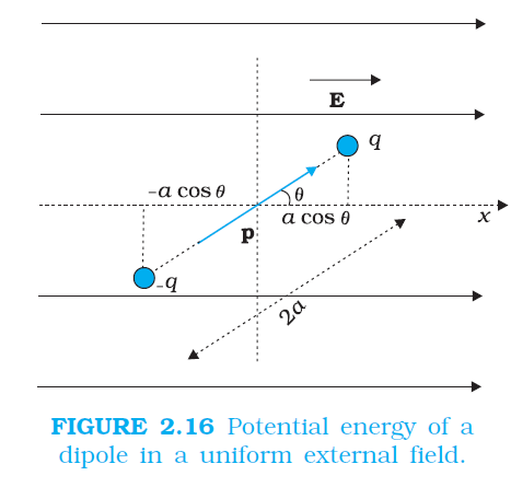
`color{blue} ✍️` Consider a dipole with charges `q_1 = +q` and `q_2 = –q` placed in a uniform electric field E, as shown in Fig. 2.16.
`color{blue} ✍️` As seen in the last chapter, in a uniform electric field, the dipole experiences no net force; but experiences a torque τ given by
`τ = p×E` ....................2.30
`color{blue} ✍️` which will tend to rotate it (unless p is parallel or antiparallel to `E`).
`color{blue} ✍️` Suppose an external torque `τ_"ext"` is applied in such a manner that it just neutralizes this torque and rotates it in the plane of paper from angle θ0 to angle θ1 at an infinitesimal angular speed and without angular acceleration.
`color{blue} ✍️` The amount of work done by the external torque will be given by
`color{green}(W = int_(theta_0)^(theta_1) τ_(ext)(theta)d theta = int_(theta_0)^(theta_1) PE sin theta d theta)`
`color{green}{= pE (costheta_0 - costheta_1)}`
...........................2.31
`color{blue} ✍️` This work is stored as the potential energy of the system. We can then associate potential energy `U(θ )` with an inclination `θ` of the dipole.
`color{blue} ✍️` Similar to other potential energies, there is a freedom in choosing the angle where the potential energy U is taken to be zero.
`color{blue} ✍️` A natural choice is to take `color{fuchsia}(θ_0 = π / 2).` (Αn explanation for it is provided towards the end of discussion.) We can then write,
`color{green}(U (theta)= pE (cos \ pi/2- cos theta) = - pE cos theta = - P*E)` ..................2.32
`color{blue} ✍️` This expression can alternately be understood also from Eq. (2.29). We apply Eq. (2.29) to the present system of two charges `+q` and `–q.` The potential energy expression then reads
`color{green}{U' (theta)=q [V(r_1)-V(r_2)] - (q^2)/(4piepsilon_0xx2a)}`
Here, `r_1` and `r_2` denote the position vectors of `+q` and `–q`. Now, the potential difference between positions `r_1` and `r_2` equals the work done in bringing a unit positive charge against field from `r_2` to `r_1.` The displacement parallel to the force is `2a cosθ`. Thus,
`color{fuchsia}([V(r_1)–V (r_2)] = –E × 2a cosθ)` . We thus obtain,
`color{green}{U' (theta)=q [V(r_1)-V(r_2)] - (q^2)/(4piepsilon_0xx2a) = - P*E - (q^2)/(4piepsilon_0)xx2a)` ..................2.34
`color{blue} ✍️` We note that `U′ (θ )` differs from `U(θ )` by a quantity which is just a constant for a given dipole.
`color{blue} ✍️` Since a constant is insignificant for potential energy, we can drop the second term in Eq. (2.34) and it then reduces to Eq. (2.32).
`color{blue} ✍️` We can now understand why we took `θ=π//2.` In this case, the work done against the external field `E` in bringing `+q` and `– q` are equal and opposite and cancel out, i.e., `color{fuchsia}{q [V (r_1) – V (r_2)]=0.}`
 (a) Determine the electrostatic potential energy of a system consisting of two charges `7 μC` and `–2 μC` (and with no external field) placed at `(–9 cm, 0, 0)` and `(9 cm, 0, 0)` respectively.